Viral adaptation is all we need? (Part 1)
Eye-opening problem of antibody synthesis.
“Bobr, kurwa” — Aleksandra (Ola) Kalisz, once, probably.
Let’s start this post by listing three random facts.
Firstly, almost two years ago, I noticed an interesting paper by Zhang et. al titled “Diffusion Models are Evolutionary Algorithms”, and later even attempted to implement it.
That's why I decided to experiment with @RobertTLange 's evojax to:
— sacha🥝 (@alexUnder_sky) November 6, 2024
1) get across with its API
2) to better understand the paper, because I liked its simple idea
preliminary notebook: https://t.co/FWfJ23Y68p
(I used Robert's code for utils and class and authors impl.) https://t.co/aZczvgPdeH
The paper was rather a thought experiment than a methodology. It mathematically proves that diffusion models inherently perform evolutionary optimisation, encompassing selection, mutation, and reproductive isolation by treating evolution as a denoising process and thus, reversed evolution as diffusion.
Secondly, a month or two before the aforementioned paper, one had been published by Oxford’s FLAIR lab “ADIOS: Antibody Development via Opponent Shaping” about evolutionaty perspective of antibody shaping (read it as a vaccine design). 1
Lastly, Dr. Rocktäschel posted several viral or not posts like one below, linking progress of reaching AGI (Artificial general intelligence, no idea what it is but people love it) with a rogue-like game NetHack.
Great post by @HenaffMikael (after ascending, what an achievement!) on what makes @NetHack_LE so extremely difficult for AI (even LLMs: https://t.co/HbKjrZGypy).
— Tim Rocktäschel (@_rockt) June 9, 2025
"While NetHack is complex in comparison to other RL benchmarks, it still contains only a tiny fraction of the… https://t.co/7QKpZrMy9y
This NetHack movement of his is really important because the benchmark’s unsolvability holds a lot of research topics (for example, Options framework, curriculum learning, hierarchical RL, open-ended RL and many more) together.
Introduction
I can bet 10 pounds that three statements confused you more than ever. This may remind you about sort of a fridge salad—just a bunch of facts without a theme, topic, or connecting idea. However, in this blogpost I will try to argue that there’s something we should solve before we make strong claims about reaching a goal or solving anything. This post is not about NetHack or how to solve it but about two its challenges, beautifully isolated in the domain of biology. Clearly, I do not fully know how to solve it (why would I). However, at the recent ICML I might have found a couple of baselines worth trying. Or not.
Viral escape as a decision-making problem
Being frank, I haven’t got any deep understanding in biology. This section is based on dialogues with AI, reading comprehension, and my coding experience with the framework.
To better understand the problem or form any sort of opinion, we need to formalise antibody shaping as an optimisation objective that can be solved numerically.
The paper claims that modern numerical methods for antibody synthesis (imagine that you design therapy to combat a scary virus like COVID-19 or, vice-versa, a scary virus that can kill everyone, like in a console game Plague) are myopic. Put simply, they take into account only current viral strain and don’t account for long-horizon mutations. Some people really felt this during the recent pandemic: such myopic synthesis of the COVID vaccines produced selective pressure on one particular viral stampp, driving its evolution toward escape variants that render the therapy ineffective.
To combat the issue ADIOS’ authors proposed a clever solution: make the problem non-stationary — continuous adaptation, which aligns with one of my previous posts, by the way) continuous adaptation. The paper frames antibody design as an iterated (repeated) two-player adversarial game between the antibody and the virus, using principles from opponent shaping in multi-agent RL. The antibody should not just be effective at the current time step; it should influence the virus’s evolutionary trajectory toward less dangerous future variants. Antibodies optimised this way were called “shapers.”
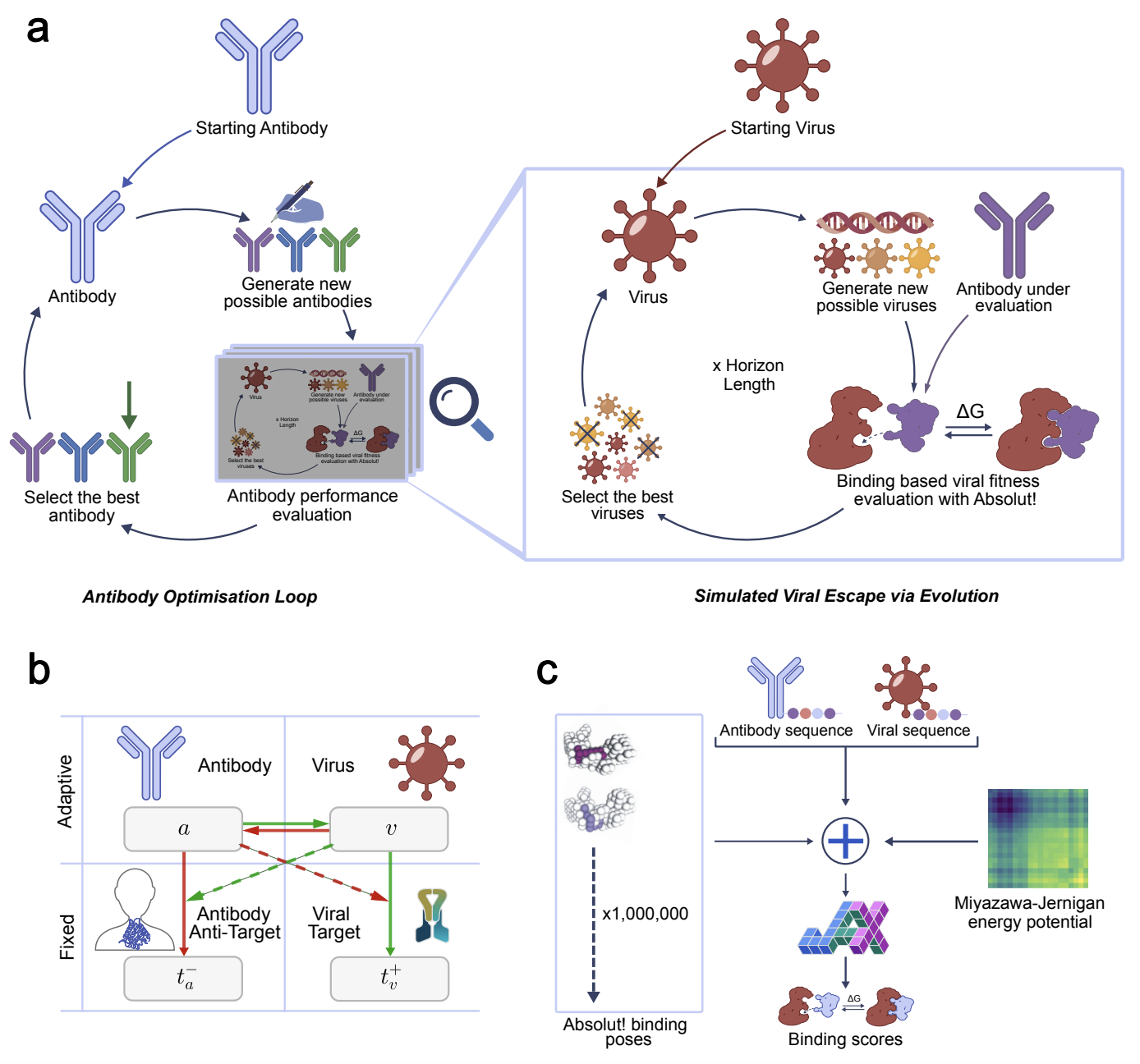
The algorithmic pipeline is shown on the picture above (panel a)). ADIOS uses nested optimisation loops (like in meta-learning):
- Inner loop (Viral Escape) simulates how the virus evolves in response to a fixed antibody over a horizon of $H$ generations. A population of viral mutants is generated, its fitness (binding escape) is evaluated using a GPU-accelerated binding simulator (Absolut!), and the fittest variants are selected. 2
- Outer loop (Antibody Optimisation): A genetic algorithm optimises the antibody to maximise performance across the entire distribution of future viral escape trajectories, not just the initial virus.
Paper is not clear about the game abstaction it uses. I might only guess but after some fights with reviewers they decided just to call the abstaction a “Markov decision process”. But it’s not completely accurate.
The paper interpets actions of the antibody $a$ and the virus $v$ as strings of nucleotides (latin letters) length $N$.
- Let $\mathcal{A}$ denote the set of 20 amino acids.
- Let $N_v$ and $N_a$ denote the sequence lengths for the virus and antibody, respectively.
- A virus action is a sequence $\mathbf{v} \in \mathcal{A}^{N_v} \in \mathbb{A}^{N_v}$.
- An antibody action is a sequence $\mathbf{a} \in \mathcal{A}^{N_a} \in \mathbb{A}^{N_a}$.
Therefore, the state of the game $\mathcal{S} = \mathcal{A}^{N_v} \times \mathcal{A}^{N_a}$ belogs to $\mathbb{A}^{N_v} \times \mathbb{A}^{N_a}$. Even given that in preliminary experiments, $N_a=N_v=11$, action space of each agent in $20^{11}=2.048\cdot 10^{14}$. Immense action space, is it not. Even for NetHack, that unsolvable benchmark, which has a context-sensitive and discrete ASCII command structur (from $93$ to $>98$ distinct actions), commitment to reinforcement learning is hard, so what can one claim about antibody shaping?
The main construction of the paper is binding (energt) strength between an antibody and a virus and it is measured by \(B: \mathbb{A}^{N_v} \times \mathbb{A}^{N_a} \to \mathbb{R}.\) Larger values correspond to stronger binding. In practice, $B(\mathbf{v}, \mathbf{a})$ is computed via the Absolut! framework as the negative of the lowest Miyazawa–Jernigan binding energy across enumerated poses (see the figure above, panels b) and c)).
To compute reward function, there (here for completeness) need to be introduced additional quantities :
- $\mathbf{t}^-_a \in \mathcal{A}^{N_a}$ : the antibody anti-target (a human protein the antibody should avoid binding to).
- $\mathbf{t}^+_v \in \mathcal{A}^{N_v}$ : the virus binding target (the host-cell receptor the virus must preserve binding to).
Furthermore, the payoffs for the antibody and the virus are defined as follows (see the figure, panel b))
Antibody payoff: the antibody aims to bind the virus while avoiding its anti-target, and implicitly penalises the virus for maintaining its infectivity target: \(R_a(\mathbf{v}, \mathbf{a}) = B(\mathbf{v}, \mathbf{a}) \;-\; B(\mathbf{t}^-_a, \mathbf{a}) \;-\; B(\mathbf{v}, \mathbf{t}^+_v)\)
Virus payoff: the virus seeks to escape antibody binding while maintaining its ability to infect host cells: \(R_v(\mathbf{v}, \mathbf{a}) = -R_a(\mathbf{v}, \mathbf{a})\)
As you can see, it’s neither pure multi-agent MDP with a Nash equilibrium (where the agents don’t want to unilatelarly deviate). It’s more of a Stackelberg game.
| Stackelberg Component | ADIOS Instantiation |
|---|---|
| Leader | The antibody |
| Leader’s action | Amino acid sequence $a \in \mathcal{A}^{N_a}$ |
| Follower | The virus |
| Follower’s response | Evolutionary trajectory $\hat{\mathbf{v}} = [\hat{v}_0, \dots, \hat{v}_H]$ |
| Leader’s objective | Maximise payoff accounting for follower’s best response: $\max_a \mathbb{E}_{\hat{\mathbf{v}} \sim E_v(\hat{v},a)}[\dots]$ |
| Follower’s objective | Maximise viral fitness (escape binding): $\max_{\hat{\mathbf{v}}} R_v(\hat{\mathbf{v}}, a)$ |
However, there is a catch. As the authors use evolutionary alogrithms and not closed-form equilibrium solvers and the viral type evolves (it doesn’t behave like a fixed entity but rather a stochastic process, possibly alternating its type), it could not be strongly classified as one—let’s call it a a Stackelberg game with an evolutionary follower.
Simulated Viral Escape (Inner Loop / Follower)
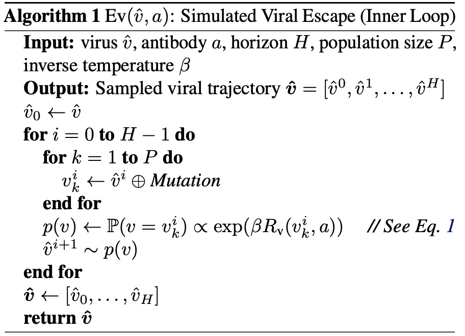
Given a fixed antibody $\mathbf{a}$ and a starting virus $\hat{\mathbf{v}}_0$, the virus evolves for $H$ generations. At each generation $i$
Generate a population of $P$ (paper uses 40) mutants (on average one amino-acid substitution per sequence) \(\mathbf{v}_i^k \;=\; \hat{\mathbf{v}}_i \,\oplus\, \text{Mutation}, \qquad k = 1,\dots,P\)
Evaluate fitness $R_v(\mathbf{v}_i^k, \mathbf{a})$ for each mutant.
Select the next generation via softmax selection: \(\Pr\!\big(\hat{\mathbf{v}}_{i+1} = \mathbf{v}_i^k\big) \;\propto\; \exp\!\big(\beta\, R_v(\mathbf{v}_i^k, \mathbf{a})\big)\)
The inner loop produces an escape trajectory distribution: \(\hat{\mathbf{v}} \;=\; [\hat{\mathbf{v}}_0, \hat{\mathbf{v}}_1, \dots, \hat{\mathbf{v}}_H] \;\sim\; E_v(\hat{\mathbf{v}}_0, \mathbf{a})\)
Antibody Fitness (Outer Loop / Leader)
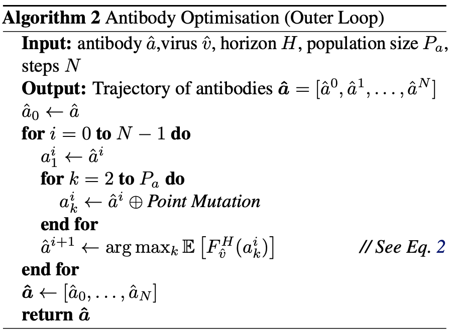
The shaper antibody is optimised against the expected performance over the entire escape horizon:
\[F^H_{\hat{\mathbf{v}}}(\mathbf{a}) \;=\; \mathbb{E}_{\hat{\mathbf{v}} \sim E_v(\hat{\mathbf{v}}_0, \mathbf{a})}\!\left[ \frac{1}{H+1}\sum_{i=0}^{H} R_a(\hat{\mathbf{v}}_i, \mathbf{a}) \right]\]The myopic baseline corresponds to the special case $H = 0$: \(F^0_{\hat{\mathbf{v}}}(\mathbf{a}) \;=\; R_a(\hat{\mathbf{v}}_0, \mathbf{a})\)
Optimisation Objective
The antibody optimiszation loop searches for the sequence that maximises the escape-averaged fitness:
\[\mathbf{a}^* \;=\; \arg\max_{\mathbf{a} \in \mathcal{A}^{N_a}} \; F^H_{\hat{\mathbf{v}}}(\mathbf{a})\]In practice, this is solved via a genetic algorithm with Monte-Carlo estimation of the expectation (drawing $\eta$ independent escape trajectories per candidate antibody).
Key results from the paper
- On Dengue virus, shapers dramatically outperform myopic antibodies in long-horizon efficacy. As the virus evolves, myopic antibodies lose effectiveness, while shapers maintain strong binding.
- Crucially, shapers don’t just resist escape, they actively steer viral evolution toward variants that are more susceptible to binding by a broad spectrum of antibodies.
- The framework works across multiple pathogens: Dengue, and some other.
- Compute Trade-offs: the authors analyse how longer planning horizons improve results but require more samples, offering practical guidance for deployment.
Takeaway?
The anti-body synthesis framework puts into absolut (no pun intended) two critical issues of modern agentic systems: long-horizon reasoning in presence of a huge action space, stripping away the transition dynamics.
In other words, the objective
- strips away all this fancy partially observable transition dynamics that RL struggles with, reducing need for careful state exploration;
- puts accent on co-improvement: the agent should be guided or controlled by another entity (or a past version of itself) to demonstrate iterative adaptaion; 3
However, as you might have noticed, the paper doesn’t use neural networks as policies’ parametrisations. Looking at the action spaces, it might be understandable why.
Nevertheless, can we try to find a solution and gain some of artificial intelligence generalisation cabilities or induced biases?
Generative models for huge action spaces
Wandering halls of the Recent ICML, I found a paper “Reinforcement Learning with Discrete Diffusion Policies for Combinatorial Action Spaces.”
Method introduced in the paper, $\text{RL-D}^2$, trains discrete diffusion models as policies for combinatorially large (ADIOS’ $20^{11}$ will do) action spaces. The action space is treated as a sequence (e.g., macro-actions in Atari, joint actions in multi-agent systems, or DNA sequences), and the diffusion model iteratively denoises a masked sequence into a high-reward action.
Combinatorial Multi-Armed Bandit
There is a single state (or the state is ignored), so the problem reduces to a combinatorial bandit.
- Let $\mathcal{A}$ be the vocabulary of nucleotides (e.g. ${\text{A}, \text{C}, \text{G}, \text{T}}$).
- An action is a DNA sequence of fixed length $K$: \(\mathbf{a} = (a_0, a_1, \dots, a_{K-1}) \in \mathcal{A}^K\)
- A reward function $r : \mathcal{A}^K \to \mathbb{R}$ predicts the desired biological property (e.g. gene expression activity).
The goal is to learn a policy $\pi_\theta$ that maximises the expected reward: \(\max_\theta \; \mathbb{E}_{\mathbf{a} \sim \pi_\theta}\!\big[\, r(\mathbf{a}) \,\big]\)
Looks pretty much as the OUTER LOOP of the ADIOS algorithm, right?
Discrete Diffusion [Preliminaries]
For a large search space, it makes more sense to perform its stochastic exploration instead of generating the sequence autoregressively (token-by-token). The policy uses an iterative denoising process—initialise a taget sequence and gradually fill it in over $N$ steps, starting from a completely blank (masked) sequence.
The Masked Forward Process
We augment the vocabulary with a special mask token: $\mathcal{A} \cup {m}$.
The forward process is a fixed noising procedure. At each diffusion step $n = 1, \dots, N$, every position in the sequence is independently either:
- kept with probability $\beta_n$, or
- masked with probability $1 - \beta_n$.
Put formally, for a single position with value $a_{n-1}^k \neq m$ 4: \(q(a_n^k = a_{n-1}^k \mid a_{n-1}^k) = \beta_n, \qquad q(a_n^k = m \mid a_{n-1}^k) = 1 - \beta_n\)
Once a position is masked, it stays masked: \(q(a_n^k = m \mid a_{n-1}^k = m) = 1\)
Noise Schedule
The values $\beta_1, \beta_2, \dots, \beta_N \in (0,1)$ form a noise schedule, typically increasing so that masking becomes more aggressive over time. A common choice are cosine or linearly annealing schedules.
Because masking is applied independently at each step, the probability that a position survives unmasked after $n$ steps is $\alpha_n = \prod_{i=1}^{n} \beta_i$.
This gives a simple closed-form for the distribution of a noised position given the original clean token $a_0^k$: \(q(a_n^k = a_0^k \mid a_0^k) = \alpha_n, \qquad q(a_n^k = m \mid a_0^k) = 1 - \alpha_n\)
So at step $n$, a position is either the original nucleotide (with probability $\alpha_n$) or a mask (with probability $1-\alpha_n$). After enough steps, $\alpha_N \approx 0$ and the sequence is almost entirely masked — pure noise.
The Learned Reverse Process
The reverse process is the generative model. Starting from a fully masked sequence $\mathbf{a}_N$ (sampled from the prior), it iteratively denoises one step at a time: \(\mathbf{a}_{N} \to \mathbf{a}_{N-1} \to \cdots \to \mathbf{a}_0\)
A neural network $f_\theta$ (in our case, it’s Transformer) looks at the current noised sequence $\mathbf{a}_n$ and step index $n$, and predicts the original clean sequence: \(\boldsymbol{\mu}_\theta(\mathbf{a}_n, n) \;\approx\; \mathbf{a}_0\)
For each position $k$, $\boldsymbol{\mu}_\theta(\mathbf{a}_n, n)$ outputs a probability distribution over the four nucleotides which is denoted by the paper’s authors as \(\mu_\theta(\mathbf{a}_n, n)_{a_0^k}\) for the predicted probability that the original clean token at position $k$ was $a_0^k$.
The policy’s sampling distribution is defined by running this reverse chain to completion: \(\pi_\theta(\mathbf{a}_0) \;=\; p_\theta(\mathbf{a}_0 \mid \mathbf{a}_N) \cdots p_\theta(\mathbf{a}_{N-1} \mid \mathbf{a}_N)\)
Training Objective (Standard ELBO)
The model is trained to reconstruct the clean sequence from its noised versions. As the full objective is intractable, standard Evidence Lower Bound (ELBO) for a single clean sequence $\mathbf{a}_0$ is used
\[\mathcal{L}_{\text{ELBO}}(\mathbf{a}_0; \theta) \;=\; -\sum_{n=1}^{N} \bar{\alpha}_n \, \mathbb{E}_{\mathbf{a}_n \sim q(\cdot \mid \mathbf{a}_0)}\!\left[ \sum_{k=0}^{K-1} \mathbb{1}\{a_n^k = m\} \cdot \log \mu_\theta(\mathbf{a}_n, n)_{a_0^k} \right]\]The formula writes as:
- We sample a diffusion timestep $n$ and a noised sequence $\mathbf{a}_n$ by randomly masking positions of $\mathbf{a}_0$ according to $q$.
- We only ask the model to predict masked positions. $\mathbb{1}{a_n^k = m}$ is an indicator that is $1$ only if position $k$ is masked at step $n$.
- $\log \mu_\theta(\mathbf{a}n, n){a_0^k}$ is the log-probability the model assigns to the true nucleotide $a_0^k$.
- $\bar{\alpha}_n$ is a weighting term derived from the schedule (it up-weights certain timesteps).
This is essentially a masked language modeling loss, but the masking pattern follows the diffusion schedule rather than being uniform.
If you prefer the language of code,
def masked_prediction_loss(
    model,
    diffusion_schedule: Array,
    a0: Array,
    cond: Array,
    rng: PRNGKey,
) -> Array:
  B, _ = a0.shape
  N = diffusion.num_steps
  rng, t_rng, noise_rng = jax.random.split(rng, 3)
  t = jax.random.randint(t_rng, (B,), 0, N)

  keep_prob = diffusion_schedule.state[t][:, None]  # (B, 1)
  mask_token = diffusion_schedule.dim - 1
  keep = jr.bernoulli(noise_rng, keep_prob, shape=a0.shape)  # (B, L)
  a_t = jnp.where(keep, a0, mask_token)
  mask = ~keep

  logits = model(a_t, t, cond, train=True)
  log_probs = jax.nn.log_softmax(logits, axis=-1)
  token_ll = jnp.take_along_axis(log_probs, a0[:, :, None], axis=-1).squeeze(-1)
  masked_nll = -jnp.where(mask, token_ll, 0.0)
  return masked_nll.sum(-1)
Policy Mirror Descent (PMD) Target
At iteration $k$, let $\pi_k$ be the current policy and let $q_{\pi_k}(\mathbf{a}) = r(\mathbf{a})$ be the action-value (reward) in the bandit setting.
The advantage could be simply defined as: \(A_{\pi_k}(\mathbf{a}) = r(\mathbf{a}) - v_{\pi_k}, \qquad v_{\pi_k} = \mathbb{E}_{\mathbf{a} \sim \pi_k}[\,r(\mathbf{a})\,]\)
The PMD update defines a target distribution $\pi_k^{\text{MD}}$ by exponentiating the advantages:
\[\pi_k^{\text{MD}}(\mathbf{a}) = \frac{1}{Z} \; \pi_k(\mathbf{a}) \exp\!\left(\frac{A_{\pi_k}(\mathbf{a})}{\lambda}\right)\]The formula above is just a straightforward solution of the RL problem in the previous section.
where $\lambda \gt 0$ is a softmax temperature and $Z = \sum_{\mathbf{a}’} \pi_k(\mathbf{a}’) \exp(A_{\pi_k}(\mathbf{a}’)/\lambda)$ is the partition function, acting as the normalisation constant.
Forward KL Divergence Objective
The paper actually considers both, forward and reverse KL optimisation problems. However, for now, I only work with the former, as it was primarily used in the DNA experiments
The new policy $\pi_{k+1}$ is obtained by minimising the forward KL from the PMD target to the parametric policy:
\[\pi_{k+1} \in \arg\min_{\pi_\theta} \; D_{\text{KL}}\!\big(\pi_k^{\text{MD}} \,\big\|\, \pi_\theta\big)\]Because this objective is intractable to minimise directly, the authors derive a tractable upper bound using the diffusion ELBO.
Intuitively, this target increases the probability of high-reward sequences and decreases the probability of low-reward sequences, while the KL term keeps the update from being too drastic. {.prompt-tip }
Discrete Diffusion Policy
There is a nice blogpost about diffusion models from Volodymyr Kuleshov’s lab. I have learnt a lot from there.
The policy $\pi_\theta$ is a masked discrete diffusion model over the sequence space $\mathcal{A}^K$.
Augmented vocabulary: $\mathcal{A} \cup {m}$ where $m$ is a mask token.
Forward KL Policy Update
The new policy $\pi_{k+1}$ is obtained by minimising the forward KL divergence from the PMD target to the parametric diffusion policy: \(\pi_{k+1} \in \arg\min_{\pi_\theta} D_{\text{KL}}\big(\pi_k^{\text{MD}} \big\| \pi_\theta\big)\)
Directly minimising this is intractable because $\pi_\theta(\mathbf{a}_0)$ requires integrating over all possible reverse diffusion paths. The key trick of RL-D² is to derive a tractable upper bound using the diffusion ELBO.
FKL Training Loss (Bandit Setting)
In the single-step (bandit) setting, the FKL objective reduces to the weighted ELBO loss. Let $\hat{\mathcal{A}}$ be a batch of sequences sampled from the current policy $\pi_k$ (via the reverse diffusion process). Then:
\[\mathcal{L}_{\text{FKL}}(\theta) \;=\; \mathbb{E}_{\hat{\mathcal{A}} \sim \pi_k}\!\left[ -\sum_{\mathbf{a}_0 \in \hat{\mathcal{A}}} w(\mathbf{a}_0) \;\cdot\; \mathcal{L}_{\text{ELBO}}(\mathbf{a}_0; \theta) \right]\]where the weights are given by a softmax over the batch advantages: \(w(\mathbf{a}_0) = \frac{\exp\!\big(\,r(\mathbf{a}_0)/\lambda\,\big)} {\sum_{\mathbf{a}' \in \hat{\mathcal{A}}} \exp\!\big(\,r(\mathbf{a}')/\lambda\,\big)}\)
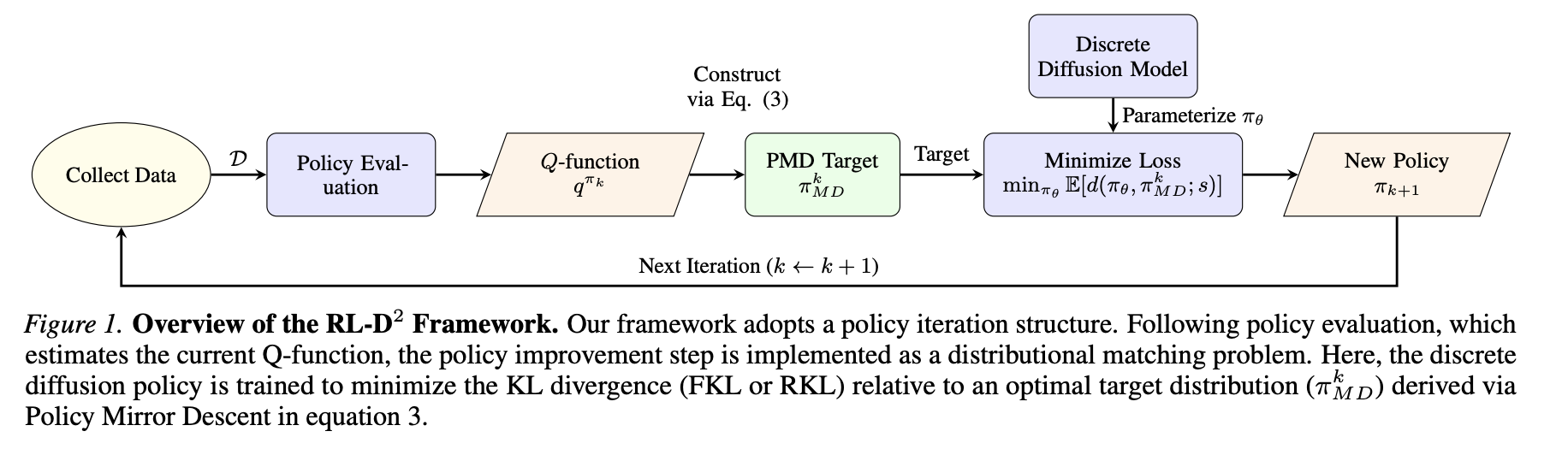
How is it approached in the paper:
- Sample a batch of nucleotide sequences from the current diffusion policy.
- Compute their rewards $r(\mathbf{a}_0)$ using the predictor.
- Reweight each sequence: high-reward sequences get larger weights.
- For each sequence, create noised versions $\mathbf{a}_n$ by masking positions according to the schedule.
- Train the model to reconstruct the original nucleotides at masked positions, but focus more on the high-reward sequences via the weights $w(\mathbf{a}_0)$.
This shifts the generative distribution toward the PMD target without ever needing to backpropagate through the sampling process.
If you prefer code,
def fkl_loss(
  model,
  diffusion_schedule: Array,
  rng: PRNGKey,
  batch: Batch,
  lambda_temp: float,
) -> Array:
  """
  batch keys:
    "actions"      : (B, L) int32
    "conditioning" : (B, C) float32 or None
    "advantages"   : (B,) float32
  """
  a0 = batch.actions
  cond = batch.conditions
  advantages = batch.payoffs

  rng, loss_rng = jax.random.split(rng)

  per_example_nll = masked_prediction_loss(
    model, diffusion_schedule, a0, cond, loss_rng
  )  # (B,)

  weights = jax.nn.softmax(advantages / lambda_temp)  # (B,)
  fkl = jnp.sum(weights * per_example_nll)
  return fkl
Algorithms
To sum up, there is a hypothesis: we can use diffusion models as large state space approximators and, therefore, switch from pure genetic algorithm formulation to first-order (gradient-based) methods of unsupervised adversarial design or opponent shaping, for example, COALA or Rational Policy Gradient.
Elitist Search (ADIOS)
1
2
3
4
5
6
7
8
9
Input: current antibody a, evaluator E, population size N
1:  candidates ← {N−1 single-point mutants of a} ∪ {a}
2:  for each candidate c in candidates (in parallel):
3:      payoff(c) ← E.evaluate(c)     // mean over num_reps independent
                                       // viral-escape simulations, each
                                       // horizon GA generations of the
                                       // antigen population vs. c
4:  a_next ← argmax_c payoff(c)
5:  return a_next
Diffusion policy as the Outer loop
1
2
3
4
5
6
7
8
9
10
11
12
13
14
15
16
17
18
19
20
21
22
23
24
25
26
27
28
29
30
State (persists across rounds): π_θ, π_old ← copy(π_θ), B ← ∅, b ← 0

Each outer round, given current antibody a:

  ── COLLECT
  1:  x ← [MASK] × antibody_length              // fully re-masked, every round
  2:  candidates ← reverse_diffuse(π_old, x, conditioning=a)
      // T denoising steps; at each step, currently-masked positions are
      // revealed with probability (ᾱ_{n-1} − ᾱ_n) / (1 − ᾱ_n); already-
      // revealed positions are never touched again (monotone unmasking)
  3:  for each candidate c in candidates (in parallel):
  4:      payoff(c) ← E.evaluate(c)             // same oracle as Algorithm 1
  5:  b ← β·b + (1−β)·mean(payoff)
  6:  for each c: advantage(c) ← payoff(c) − b
  7:  B.push({(c, a, advantage(c)) for c in candidates})   // FIFO evict if |B| > C
  8:  a_next ← argmax_c payoff(c)               // this round's own best,
                                                  // no cross-round memory

  ── UPDATE (repeated num_update_steps times)
  9:  for step = 1 … num_update_steps:
 10:      batch ← C samples drawn uniformly, with replacement, from B
 11:      weights ← softmax(advantage / λ)  over batch
 12:      for each (c, cond, _) in batch:
 13:          mask ← Bernoulli(1 − ᾱ_t) per position, t ~ Uniform(0, T)
 14:          nll(c) ← −log π_θ(c | mask(c), cond)  summed over masked positions
 15:      loss ← Σ_batch  weight · nll
 16:      θ ← θ − ∇_θ loss                      // Adam step
 17:      every target_update_freq steps: π_old ← copy(π_θ)

  return a_next
Steps 1-2 regenerate the entire sequence from scratch every round, conditioned only on a through the denoiser’s learned attention to it, so there is no structural guarantee, the way the algorithm’s mutation operator has, that a candidate stays close to the current incumbent.
Current experimental plan
CODE is located here: https://github.com/alexunderch/adios
We use a simple (2 layers) diffusion transfomer with additional (and optional) FiLM antibody conditining for preliminary experiments. For now, we mostly stick to ADIOS implementation setting and its current hyperparameters (until I don’t become better at biology).
We experiment with the following biological parameters (Dengue virus, PDB code 2R29, antibody length is fixed and equal to 11):
1
2
3
viral_target = "CARLVQLGLYY"
antigen = "SYSMCTGKFKVVKEIAETQHGTIVIRVQYEGDGSPCKIPFEIMDLEKRHVLGRLITVNPIVTEKDSPVNIEAEPPFGDSYIIIGVEPGQLKLNWFKK"
antibody_antitarget = "GRFLVNLQAKKDREAWYYWGPWNKAYWFSDPGMFDPWKQAEQSYFCNANPVCYAEHFMLGPITQKTPMVYHDPEPSKGGCVTVHNNATDYIMPDCYN"
First failed attempts
Just running a $\text{PM-D}^2$ optimisation yields the following results.
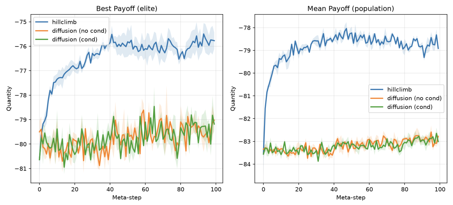
We must notice that although diffusion models are steadily improving, they are yet much worse than plain evolutionaty optimisation with genetice algorithm. It’s also unclear if additional conditioning is worth it. Clearly, in agreement with the note above, exploration process stays too stochastic, and it generates low quality data putting the model’s success more on luck than on an inductive bias.
Reverse sampling generalisation
As I have noticed that the model doesn’t necessarily have to improve to generate better sequences, I decided to “help the model” to recover good sample, analogous to teacher forcing in autoregressive models.
def local_sample_reverse(
  rng: PRNGKey,
  model,
  diffusion_schedule: Array,
  conditioning: Array,
  incumbent: Array,
  num_samples: int
  antibody_length: int,
  noise_level: int,
) -> Array:

  rng, mask_rng = jr.split(rng)
  keep_prob = diffusion_schedule.state[noise_level]
  keep = jax.random.bernoulli(mask_rng, keep_prob, shape=(num_samples, antibody_length))
  mask_token = diffusion_schedule.dim - 1
  x0 = jnp.where(keep, incumbent[None, :], mask_token)

  def step(carry, n):
    x, rng = carry
    rng, model_rng, reveal_rng = jr.split(rng, 3)
    t = jnp.full((x.shape[0],), n, dtype=jnp.int32)
    logits = model(x, t, conditioning, train=False)
    preds = jr.categorical(model_rng, logits, axis=-1)
    is_masked = x == mask_token
    state_n    = diffusion_schedule.state[n + 1]
    state_prev = diffusion_schedule.state[n]
    p_reveal = jnp.where(
      state_n < 1.0, (state_prev - state_n) / (1.0 - state_n), 1.0
    )
    reveal_now = jax.random.bernoulli(reveal_rng, p_reveal, shape=x.shape) & is_masked
    return (jnp.where(reveal_now, preds, x), rng), None

  (x_final, _), _ = jax.lax.scan(
    # not over the full sequence!
    step, init=(x0, rng), xs=jnp.arange(noise_level), reverse=True
  )
  return x_final
You can observe comparison between global baseline sampling and new version in Table below.
| Aspect | Global Sampling (Baseline) | Local sampling |
|---|---|---|
| Starting state | Fully masked ([MASK] × L), every round | Incumbent partially re-masked to noise_level; unmasked positions guaranteed equal to incumbent |
| Locality guarantee | None — only via learned attention to conditioning | Structural, by constructionsame mechanism hillclimb’s mutation operator relies on |
| Denoising sub-task difficulty | Fill in all L nucleotide positions jointly from nothing | Fill in only the re-masked positions (~30-40%), conditioned on the rest being correct |
| Relationship to model-collapse risk | Fully self-consuming loop (π_old generates → π_θ trains on that output → resync) with no external grounding each round | Each round’s candidates anchored to a position chosen by real evaluation (the incumbent); closer to injecting fresh, grounded data every generation |
| Inherited failure mode | Full-space search, in principle immune to single-mutation local optima | Likely inherits hillclimb’s own weakness: small fixed neighbourhoods can’t cross valleys needing simultaneous multi-position changes |
Consensus mode: local sampling with annealed noise_level $n(t)$ , conversing to the global version—a competence curriculum.
where
\[\begin{aligned} k(t) = k_{\min} + (k_{\max} - k_{\min})\,\min\!\left(\frac{t}{T_{\text{warm}}},\, 1\right), \\ n^*(k) \;=\; \min\Bigl\{\, n \in \{1,\dots,N-1\} : \bar{\alpha}_n \leq 1-\frac{k}{L} \,\Bigr\}, \end{aligned}\]$L$ is the antibody length, $T_{\text{warm}}$ is a number of warmup steps. The schedule controls the sequence edit budget $k(t) \in [k_{\min}; k_{\max}]$, which varies from strong locality (point-wise mutations) to broader exploration. The schedule is implemented in a way that expected Hamming distance to from the incumbent stays as close to the bucket $k(t)$ at each time step $t$.
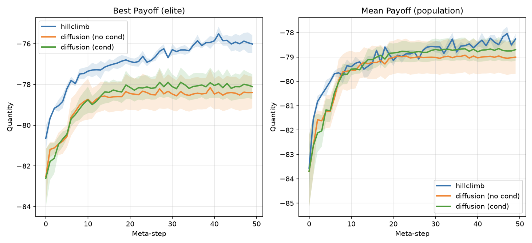
As can be observed, if we apply only local mutation, the results become immediately better but 1) still worse than a simple evolutionary baseline; 2) doing only point-wise mutations, we “waste” a lot of generalisation capabilities of the diffusion models. This experiment just shows that one of the things we should care about is controllability of the mutation in the huge design space.
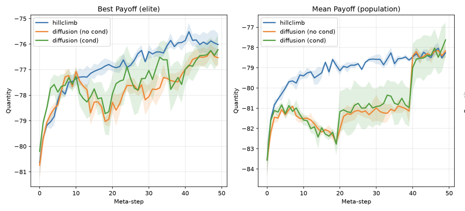
With an heuristical schedule ($T_\text{warm}$, $k_{\min}$, $k_{\max}$ and fixed horizn $H=10$) the diffusion peforms competitively with the evolution—what we actually needed.
| Algorithm | Verif. perf | Gap (best-mean) |
|---|---|---|
| Hillclimb | -82.7 ± 0.5 | -2.5 |
| Diffusion | -79.8 ± 0.4 | -3.1 |
| Diffusion w/ cond. | -81.3 + 0.4 | -1.8 |
Diffusion is clearly better than evolution on validation. However, as I used only 3 seeds, I don’t think that we can do a statistically significant prediction.
Increading the horizon (up to $H=50$) improves the performance.
Therefore, it’s mostly about how you explore in the strategy space when performing reverse sampling with the diffusion model. Current goal is to lessen number of hyperparameters, or decision “knobs”, making the noise level schedule likelihood (or ELBO)-dependent.
Current conclusions
Antibody shaping is a very interesting problem, perfectly isolating major issues of the current agentic and RL systems. Solving it with neural networks would bring us as much value as optimising for a lot of other RL benchmarks. Thus, I currently proposed a method that uses generative models. Currently not that successful, being honest, but I think I am on the right way and eager to prove it.
Special shoutout
goes to Options framework as a way to scalably tackle problems of hierarchical RL; macro actions used in $\text{RL-D}^2$ could be viewed as a reinstantiation of options. Therefore, they might be that missing piece to solve the whole problem. I want to point out a recent paper.
Scalable Option Learning (SOL) addresses the scalability challenge that both $\text{RL-D}^2$ and ADIOS face: how to train policies that reason over long horizons in combinatorial spaces. SOL scales option learning (hierarchical RL) to 30 billion frames on NetHack, achieving ~35× higher throughput than prior hierarchical methods.
Thank you for reading if you are interesting in this kind of problem and have one GPU to use, don’t hesitate to contact me.