An example where collective intelligence helps

“I absolutely love toy experiments” — Jeffrey Seely.

Nowadays, reinforcement learning (RL) serves as a predominant paradigm in training or finetuning of decision-making systems in pretty much field of science or industry, partly because of adoption of RL environments. One of the maintainers, Will Brown, gave nice advice to people whose runs didn’t really converge — “increase batch size.”

keep learning rate on the lower side, don't make your batch size too small, vary your system prompt and/or tools within the train set, consider adding some other envs to the train mix at lower proportions for diversity, monitor online eval performance for other tasks

— will brown (@willccbb) March 6, 2026

Of course, I meme here a tad. Nevertheless, big batches empirically help with an accurate gradient estimation when training RL algorithms. This observation covers almost all deep RL demos: Atari, MuJoCo, Control applications — pretty much all of them use replay buffers, some methods (for instance, PQN) are even based on massive parallelisation as the first class citizen.

However, let’s consider an edge-case — batch size equal to one. It’s also called “streaming” RL, or incremental RL. These algorithms despite being not that GPU-trendy are mostly focused on resource-constrained (embedded) applications or—wonderfully—in Artificial Life (ALife) and physical simulations where reducing batch-collection latency is essential for the system’s goals.

This piece is inspired by a nice conversation with @Ciaran from Sakana and his work on ALife.

Streaming barrier

I won’t act as an expert and just list three obvious reasons why it’s so tough to make streaming RL work:

• You can’t pause the world to compute a batch gradient
• Memory is constrained (small networks, no replay)
• The environment is non-stationary by design

One of recent papers—”Streaming Deep Reinforcement Learning Finally Works” by Elsayed et al.’s—addresses this via adding back eligibility traces, baselines, introducing normalisation and overshooting (lookahead) to the optimisation to empirically reduce variance of the updates in various RL algorithms. However, Elsayed et al. show the barrier is deeper: it’s about representation collapse, target network instability, and optimiser state divergence in deep nets. The variance acts really as a symptom, not the root cause. ¹

The uncomfortable truth (trvthnuke): even with perfect baselines and variance reduction, streaming deep RL can fail because the optimisation dynamics themselves become unstable and proved to work only empirically.

At the recent ICML I saw a couple papers that tried to address the problems: ²

1. Introducing baselines, however, the estimate states noisy, therefore, doesn’t actually reduce anything
2. Eligibility traces average over time, but in non-stationary environments (the Alife regime or recommendation systems), old gradients become biased and can’t fully stabilise the updates
3. Self-prediction (BYOL-RL, SPR) stabilises representations but doesn’t approach the gradient variance itself. Also, some of the methods cheat on using bigger batch sizes to establish accurate representations.

So, what’s next?

Collective escape

Remember that it’s just a proposition: artificially complicate the problem’s structure to enrich the problem set.

Let’s commit to surprise move and move out of the comfort zone. Why am I so focused on Alife applications. Isn’t it boring—just iterate your cellular automata and call this art? Bullshit. Artificial life gives sends us a hint: flocks, ant colonies, bacterial swarms, societies—agents don’t usually learn in isolation. They’re embedded in a collective. Here I can start waffling about equilibria and the problem structure. But not this time—we go for a different abstraction.

Making problem multi-agent combinatory enriches the solution space. Usually, it’s a problem we want to avoid. Not this time. Problem structure suits for distributed optimisation over a shared landscape (the task space the aims to solve), where each agent (ant) is a noisy gradient sampler and the collective (colony) is a variance-reduction device.

Let’s illustrate the problem on the simplest example, Decentralised Stochastic Gradient Descent (D-SGD). ³

We work with $n$ agents indexed by $i\in{1, \ldots, n}$. Each agent maintains local parameters $\theta^i\in\mathbb{R}^d, d>1$. The agents are arranged into a communication graph, an undirected graph $G=(V, E)$, where $V={1, \ldots, n}$. Agents can observe each other iff $i, j\in V \to (i, j) \in E$.

The system is equipped with a doubly stochastic Mixing (topology) Matrix $W \in \mathbb{R}^{n\times n}$ ($W\mathbf{1} = \mathbf{1}$, $W^\top\mathbf{1} = \mathbf{1}$, rows and columns sum to 1) that respects the graph topology: $W_{ij}=1$ iff $(i, j) \in E$ or $i=j$.

Each agent has a local scalar objective $f^i : \mathbb{R}^d \to \mathbb{R}$ (your favourite standard RL objective). The global objective is: \(f(\theta) = \frac{1}{n}\sum_{i=1}^n f^i(\theta_i).\)

At time step $t$, agent $i$ observes a noisy gradient: \(g_i^t = \nabla f_i(\theta_i^t) + \xi_i^t,\)

where $\mathbb{E}[\xi^t_i]=0$ and the noise is independent across agents: $\mathbb{E}[\xi_i^t \cdot \xi_j^t] = 0$ for $i\neq j$.

To update own weights, each agent performs ⁴

\[\theta_i^{t+1} = \sum_{j\in\text{Neighbours}(i)} W_{ij} \theta_j^t - \eta \cdot g^t_i.\]

Additionally, the method puts two critical assumptions on the collective:

1. $\frac{1}{n}\sum_{i=1}^n |\nabla f_i(\theta_i) - \nabla f(\theta)|^2 \leq \zeta^2, \quad \forall \theta$. $\zeta$ measures how different agents’ local problems are. In our Alife setting it is small when neighbours face similar subproblems (smooth landscape) and large when they don’t (patchy environment, competition).
2. Spectral gap (1 - the second largest eigenvalue) of $W$ is bounded between 0 and 1, staying bounded away from zero. It measures connectivity and shortly requires some interaction to be present.

Topology	$\rho$ (approx)	Mixing time	Variance reduction
Complete graph	$1$	$O(1)$	$n\times$
Random expander	$O(1)$	$O(\log n)$	$n\times$
2D grid	$O(1/n)$	$O(n)$	$\sim n$ (slow mixing)
Ring	$O(1/n^2)$	$O(n^2)$	$\sim n$ (very slow)

Pay attention to the fact that $\rho$ doesn’t vanish as the network grows or as topology gets sparse.

Why bother?

Here I make claims based on the proofs I found in the papers

The method has a provable variance decomposition bound (source):

\[\mathbb{E}\|g_i^{\text{eff},t}\|^2 \leq \underbrace{\sigma^2 \sum_j W_{ij}^2}_{\text{spatial averaging}} + \underbrace{\zeta^2}_{\text{heterogeneity bias}}\]

If we have uniform $k$ neighbour mixing, $\sum_j W_{ij}^2 = 1/k$, giving $k$ fold variance reduction from the consensus step alone.

D-SGD provides the following bias-variance tradeoff on the gradient update (source):

\[\text{Var}(g_i^{\text{corrected}}) \approx \frac{\sigma^2}{k} + O\left(\frac{\zeta^2}{\rho^2}\right)\]

you reduce local variance by $1/k$ but pay $\zeta^2/\rho^2$ in consensus bias.

Collective D-SGD outperforms independent SGD when (derivation uses sources above plus source) \(\frac{\sigma^2}{k} + \frac{\zeta^2}{\rho^2} < \sigma^2,\)

or put simply, the collective reduces the variance when local disagreement (ζ) is small relative to local noise (σ) and graph connectivity (ρ).

There is no complete convergence proof for D-SGD in non-stationary policy gradient learning. The guarantee above holds for the optimisation layer. The RL dynamics: exploration, representation learning, non-stationarity remain empirical.

The intuition could be formalised in a form of pseudocode

1. Each agent gets a noisy gradient: g_i = ∇f(θ_i) + ξ_i where ξ_i ~ N(0, σ²I) 
2. The noise is INDEPENDENT across agents: E[ξ_i · ξ_j] = 0 for i ≠ j 
3. Collective RL reduces variance by averaging over the population through consensus step: 
θ_i ← Σ_j W_ij θ_j. This implicitly averages independent noise realizations → Variance drops by factor ~k (neighbourhood size) 
4. The displacement d_i = θ̄_i (population mean) - θ_i encodes the accumulated difference between local and neighbourhood gradients. It acts as an implicit control variate. 
5. The update: 
θ_i ← θ_i - η · [g_i + β · (θ̄_i - θ_i)/η] 
local step + consensus correction

The method could be related to neuroscience (not as baseless):

• Neuromodulation as adaptive mixing: dopamine doesn’t just signal reward; it signals surprise relative to the collective. The modulation strength is the $\beta$ coefficient.
• Social learning as consensus: birds in a flock don’t compute average headings explicitly; they align locally, and thus emerge the population statistics.

Have we really done it?

Not really. Collective learning doesn’t eliminate the bias-variance tradeoff in updates, it factorises it. Instead of trading temporal bias (stale gradients) for variance reduction, we trade spatial bias (neighbour disagreement) for variance reduction. This is where a collective topology comes in: neuromodulation of how the agents agreed/disagreed acts as a good variance estimator.

Toy experiment

Code is released below:

We test whether a collective of streaming RL agents can overcome the variance floor that traps single-agent learners. For this, we use CartPole-v1 as a testbed, but keep the mechanism general: spatial variance reduction via decentralised consensus.

We use a baseline Stream AC with ObGD (Elsayed et al., 2024).

We test three conditions:

• Independent: 4 agents learn alone, no communication. This is the stream-barrier baseline.
• Shared: 4 agents periodically copy the parameters of a single “leader.” This is the centralised oracle: it shows the best possible variance reduction if you could synchronise perfectly.
• D-SGD: 4 agents mix parameters via a ring-topology (because why not) consensus matrix every 100 steps. No leader, no gradient sharing, only local parameter averaging.

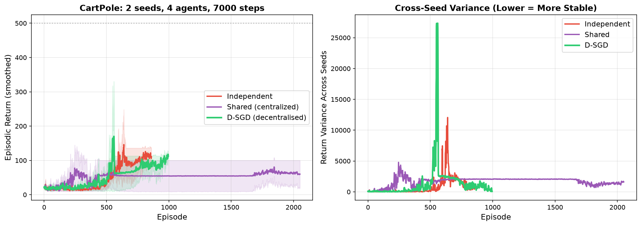
In our toy experiment, the centralised baseline (Shared) converges to a stable but mediocre policy and never escapes. Independent agents explore more but suffer from sustained high variance, the outcome is not reproducible across seeds. D-SGD shows a distinctive pattern: a burst of cross-seed variance as different agents discover different strategies, followed by a collapse as local consensus. The result is higher peak performance than either extreme, with lower sustained variance than independent learning. The collective doesn’t just reduce noise, it may turn exploration into a reproducible, stabilisable process.

We used much less episodes (100 times less than in original paper) and only 3 seeds, so may have to run more, if to convert to some paper-worth results.

Outro

Single-agent streaming RL hits a barrier: variance is too high to converge reliably, and a set of standard fixes— baselines, eligibility traces, self-prediction—either doesnt’t help or makes things worse. The uncomfortable truth is that this is that me we might hit a limit for one learner. However, if we deliberately make a problem collective—even a decentralised one with only local observation—the agents can use each other’s parameter trajectories as implicit control variates.

The consensus step in distributed SGD averages independent noise realisations across space, not time. This reduces variance by a factor of neighbourhood size without requiring memory, replay, or explicit gradient sharing. The cost is spatial bias: you need neighbors facing similar subproblems. The gain is breaking the stream barrier that single agents cannot cross.

If the idea is interesting you may apply different decentralised methods or actually look at the RL convergence guarantees. Cheers!

1. Backward view on TD-optimisation: see https://arxiv.org/abs/2007.01839. ↩︎

2. https://icml.cc/virtual/2026/poster/64761, https://icml.cc/virtual/2026/poster/62516 ↩︎

3. Decentralised (federated) optimisation is a very nicely explored field, you can get familiar with different methods like SCAFFOLD (Stochastic Controlled Averaging), Push-Sum Protocol (For Directed/Asymmetric Topologies), ADMM, Gradient tracking solutions and many many other methods. ↩︎

4. For those boring people, we assume that 1) Each $f^i$ is $L$-smooth; 2) $\mathbb{E}|g_i^t - \nabla f_i(\theta_i^t)|^2 \leq \sigma^2$ (local variance is bounded, which is a strong but illustrative assumption) ↩︎